Visually Shaping TrafPy Distributions
Up until now you have assumed you already knew all the parameters of each distribution you have generated with TrafPy. But what if you want to replicate a distribution which has either not been produced in TrafPy before or has not had open-access data provided? TrafPy has a useful interactive Jupyter-Notebook which integrates with all of the above functions, allowing distributions to be visually shaped. Crucially, once a distribution has been shaped, it can be easily replicated with TrafPy so long as the set of parameters used to shape the distribution are shared.
Academic papers present network traffic distribution information in many forms. It could be e.g. a plot, an analyticaly described named distribution (e.g. ‘the connection duration times followed a log-normal distribution with mu -3.8 and sigma 6.4’), an analytically described unnamed distribution (e.g. ‘the flow sizes followed a distribution with minimum 8, maximum 33,000, mean 6,450, skewness 1.23, and kurtosis 2.03’) etc.
The TrafPy Jupyter Notebook tool enables distributions to be tuned visually and analytically to reproduce literature distributions. Distribution plots are live-updated as slide bars, text boxes etc. are adjusted, with analytical characteristics of the generated distributions continuously output to aid accuracy.
Navigate to the directory where you cloned TrafPy and launch the Jupyter Notebook:
$ jupyter-notebook main.ipynb
The Notebook has a few main sections with markdown descriptions for each:
Import
trafpy.generatorSet global variables
Generate random variables from ‘named’ distribution
Generate random variables from arbitrary ‘multimodal’ distribution
Generate discrete probability distribution from random variables
Generate random variables from discrete probability distribution
Generate source-destination node distribution
Use node distribution to generate source-destination node demands
Use previously generated distributions to create single ‘demand data’ dictionary
Generate distributions in sets (extension)
All of the above sections can be used together or independently depending on which functionalities you need to shape your specific distribution. Below are demonstrations of how to use the interactive distribution-shaping cells.
Note
To run a Jupyter Notebook cell, click on the cell and click ‘Run’ on the top ribbon.
If you are running a cell with a TrafPy interactive graph, some configurable parameters
will appear. Adjust these parameters and click the Run Interact button to update
your plot (and the returned values).
Note
Once you have shaped your distribution, you can simply plug your shaped parameters into the previously described functions to generate your required random variable data/distributions in your own scripts. I.e. There is no need to have to save your Notebook data if you note down your shaped parameters and enter them into your own TrafPy scripts.
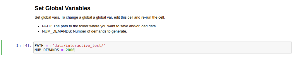
Set Global Variables
Set the PATH global variable to the directory where you want any data generated with the Notebook
to be saved. You can also set the NUM_DEMANDS global variable, which will ensure
that each time you shape a distribution for a certain traffic demand characteristic,
the correct number of demands will be generated.
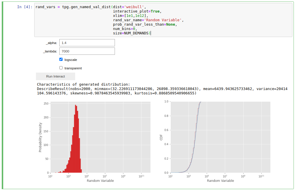
Generate Random Variables from ‘Named’ Distribution
Use this section to shape the previously described ‘named’ value distributions
(Pareto, Weibull, etc.) generated by trafpy.gen_named_val_dist().
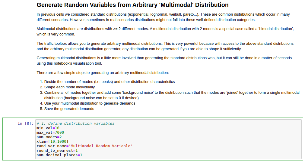
Generate Random Variables from Arbitrary ‘Multimodal’ Distribution
Use this section to shape the previously described ‘multimodal’ value distribution
generated by trafpy.gen_multimodal_val_dist().
There are a few steps to generating a multimodal distribution with TrafPy:
Define the random variables of your multimodal distribution. Set the minimum and maximum possible values, the number of modes, the name of your random variable, the x-axis limits, what to round the values to, and how many decimal places to include. Run the 1st cell.
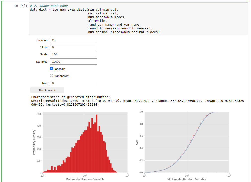
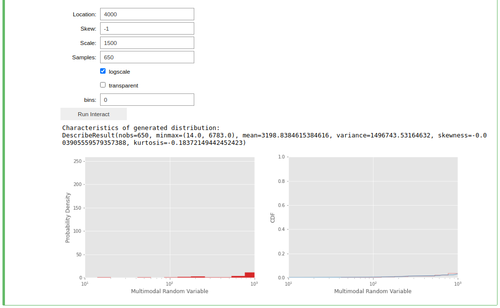
Run the 2nd cell to launch the visualisation tool. A set of tuneable parameters for each mode (where you specified
num_nodesin the previous cell) will appear. Adjust the parameters and clickRun Interactuntil you are happy with the shape of each mode. UseLocationfor the mode position,Skewfor the mode skew,Scalefor the mode standard deviation,Samplesfor the height of the mode’s probability distribution, andbinsfor how many bins to plot (default of 0 automatically chooses number of bins).
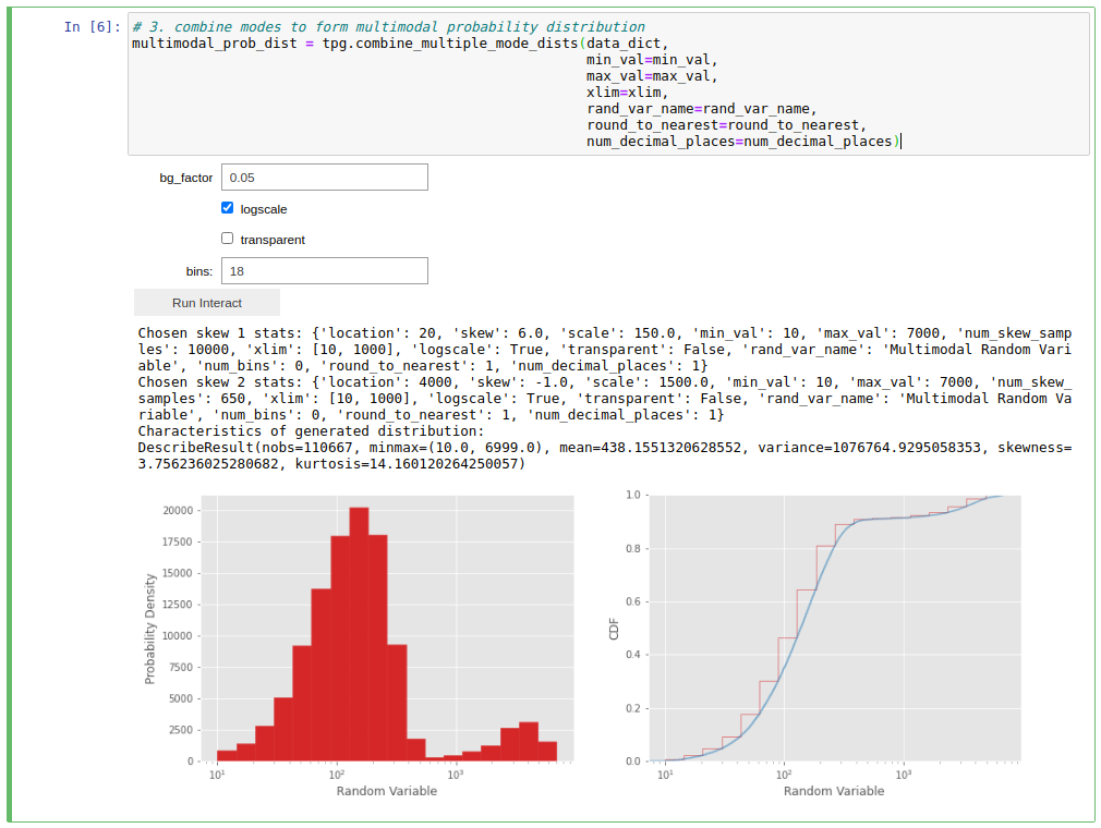
Run the 3rd cell to combine the above modes. Adjust
bg_factorto increase or decrease the ‘background noise’ amongst your shaped nodes.
Note
You may find it useful to jump between the 2nd and 3rd cells to improve the accuracy of the modes relative to one-another.
(Optional) Run the 4th cell to use your shaped multimodal distribution to sample random variable data.
(Optional) Run the 5th cell to save your mutlimodal random variable data