Job-Centric Traffic Demands
>>> import trafpy.generator as tpg
A job is a task sent to a network (such as a data centre) to execute. Jobs are computation graphs made up of operations (ops). Jobs might be e.g. a Google search query, generating a user’s Facebook feed, performing a TensorFlow machine learning task (e.g. backpropagation), etc.
In this context, an op is a data process ran on some machine where the result is specified by a pre-determined rule/programme. Each op requires >= 0 tensors/data objects as input, and produces >= tensors as output.
In a job computation graph, if an op v requires >= 1 input(s) produced by op u, the ops will be connected by a directed edge, [u, v], representing the dependency between the two ops. The edge attributes here are features of the tensor (e.g. size, source machine, destination machine, etc.).
In a data centre, when a job arrives, each op in the job is placed onto some machine to execute the op. These ops might be placed all on one machine or, as is often the case for many applications, spread out across different machines in the network according to e.g. some heuristic. The network is used to pass the tensors around between the machines executing the ops. These tensors/data objects flowing between ops are flows. The flows of a given job might flow through the network at the same time or at different times depending on e.g. scheduling decisions, constraints, dependencies, etc.
Note
In a job graph, edges between ops represent 1 of 2 types of op dependency:
Data dependency: Op j can only begin when op i’s output tensor(s) have arrived. Therefore, data dependencies become network flows if op j and op i are ran on separate network endpoints.
Control dependency: Op j can only begin when op i has finished. No data is exchanged, therefore control dependencies never become network flows.
Common job demand characteristics include:
job interarrival time;
which machine each op in the job is placed on;
number of ops in the job;
run times of the ops;
size of data dependencies (flows) between ops;
ratio of control to data dependencies in job computation graph; and
connectivity of job graph.
You can use the same value and node distributions as before to generate realistic
job demands. The only difference is that now you will pass additional arguments
into tpg.create_demand_data(). TrafPy will respond by generating job computation graphs
rather than flows as the demands in the returned dictionary.
Consider that you want to create 10 realistic data centre jobs in the same simple
5-node network as before (but now omitting show_fig to save page space).
>>> network = tpg.gen_simple_network(ep_label='endpoint')
>>> network_load_config = {'network_rate_capacity': network.graph['max_nw_capacity'], 'ep_link_capacity': network.graph['ep_link_capacity'], 'target_load_fraction': 0.1}
You could start by definiing the flow size distribution of the flows inside the job graphs
>>> flow_size_dist = tpg.gen_multimodal_val_dist(min_val=1,max_val=100,locations=[50],skews=[0],scales=[10],num_skew_samples=[10000],bg_factor=0,round_to_nearest=1,num_bins=34)
then the job interarrival time distribution
>>> interarrival_time_dist = tpg.gen_multimodal_val_dist(min_val=1,max_val=1e8,locations=[1,1,3000,1,1800000,10000000],skews=[0,100,-10,10,50,6],scales=[0.1,62,2000,7500,3500000,20000000],num_skew_samples=[800,1000,2000,4000,4000,3000],bg_factor=0.025,round_to_nearest=1)
then the number of ops in each job
>>> num_ops_dist = tpg.gen_multimodal_val_dist(min_val=50,max_val=200,locations=[100],skews=[0.05],scales=[50],num_skew_samples=[10000],bg_factor=0.05,round_to_nearest=1)
and then the source-destination node (i.e. op machine placement) distribution
>>> endpoints = network.graph['endpoints']
>>> node_dist = tpg.gen_multimodal_node_dist(eps=endpoints,num_skewed_nodes=1)
You can then use your distributions to generate your job-centric demand data returned neatly into a single dictionary:
>>> job_centric_demand_data = tpg.create_demand_data(eps=endpoints,node_dist=node_dist,flow_size_dist=flow_size_dist,interarrival_time_dist=interarrival_time_dist,num_ops_dist=num_ops_dist,c=1.5,max_num_demands=10,network_load_config=network_load_config,use_multiprocessing=False)
Don’t forget to save your data:
tpg.pickle_data(data=job_centric_demand_data,path_to_save='data/job_centric_demand_data.pickle',overwrite=True,zip_data=True)
TrafPy job-centric demand data dictionaries are organised as:
{
    'job_id': ['job_0', ..., 'job_n'],
    'job': [networkx_graph_job_0, ..., networkx_graph_job_n],
    'event_time': [event_time_job_0, ..., event_time_job_n],
    'establish': [event_establish_job_0, ..., event_establish_job_1],
    'index': [index_job_0, ..., index_job_1]
}
Where the 'job' key contains the list of job computation graphs with all
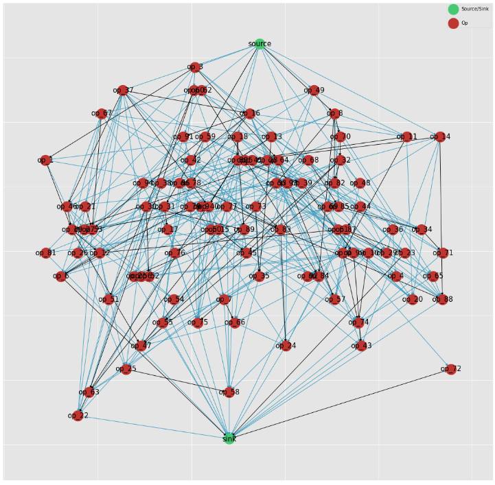
the embedded demand data. You can visualise the job computation graph(s):
>>> jobs = list(job_centric_demand_data['job'][0:2])
>>> fig = tpg.draw_job_graphs(job_graphs=jobs,show_fig=True)